Web scaping

Lecture 10

Dr. Mine Çetinkaya-Rundel

Duke University
STA 199 - Fall 2024

October 1, 2024

Warm-up

While you wait…

If you haven’t yet done so: Install a Chrome browser and the SelectorGadget extension:
- Chrome
- SelectorGadget
Go to your ae project in RStudio.
Make sure all of your changes up to this point are committed and pushed, i.e., there’s nothing left in your Git pane.
Click Pull to get today’s application exercise file: ae-10-chronicle-scrape.qmd.
Wait till the you’re prompted to work on the application exercise during class before editing the file.

Announcements

Midterm things:

Practice midterm: Posted on the course website
Lecture recordings: Available until the in-class midterm, link emailed earlier today
Application exercise catch-up: Complete all application exercises up to the midterm by the in-class midterm (and get any missed points!)
Midterm review: In class on Thursday, come with questions!

From last time

Age gaps

Data prep:

library(tidyverse)

age_gaps <- read_csv("data/age-gaps.csv")

age_gaps_heterosexual <- age_gaps |>
  filter(character_1_gender != character_2_gender)

Age gaps

Label the data:

age_gaps_heterosexual <- age_gaps_heterosexual |>
  mutate(
    older = case_when(
      character_1_gender == "woman" & actor_1_age > actor_2_age ~ "woman older",
      character_2_gender == "woman" & actor_2_age > actor_1_age ~ "woman older",
      character_1_gender == "man"   & actor_1_age > actor_2_age ~ "man older",
      character_2_gender == "man"   & actor_2_age > actor_1_age ~ "man older",
      actor_1_age == actor_2_age ~ "same age"
    )
  )

Age gaps

Age gaps split:

woman_older <- age_gaps_heterosexual |> 
  filter(older == "woman older")
man_older   <- age_gaps_heterosexual |> 
  filter(older == "man older")
same_age    <- age_gaps_heterosexual |>
  filter(older == "same age")

Check:

(
  nrow(woman_older) + nrow(man_older) + nrow(same_age)
) == nrow(age_gaps_heterosexual)

[1] TRUE

Age gaps

Write data

write_csv(woman_older, file = "data/woman-older.csv")
write_csv(man_older, file = "data/man-older.csv")
write_csv(same_age, file = "data/same-age.csv")

Data on the web

Reading The Chronicle

How often do you read The Chronicle?

Every day
3-5 times a week
Once a week
Rarely

Reading The Chronicle

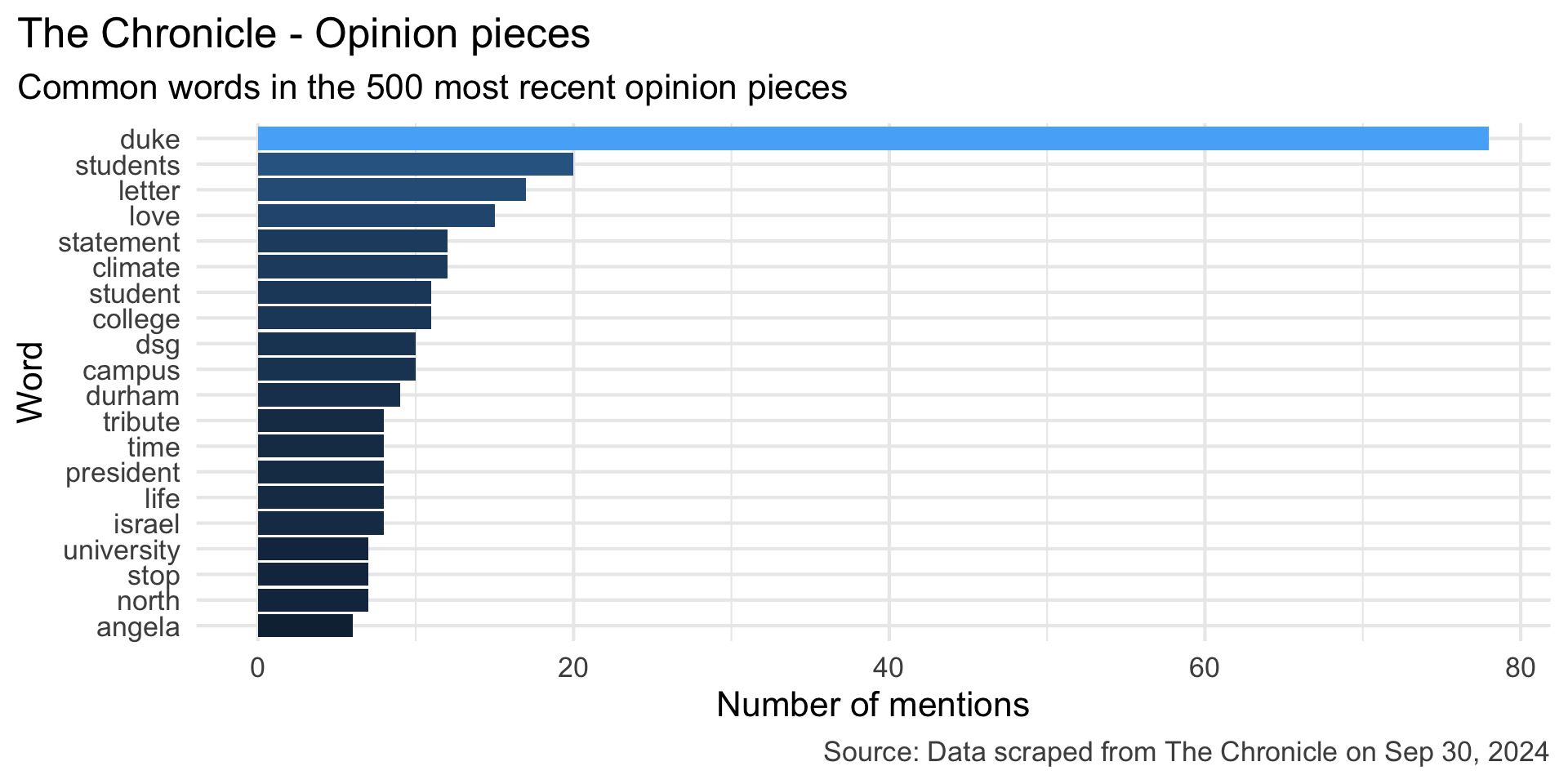
What do you think is the most common word in the titles of The Chronicle opinion pieces?

Analyzing The Chronicle

Reading The Chronicle

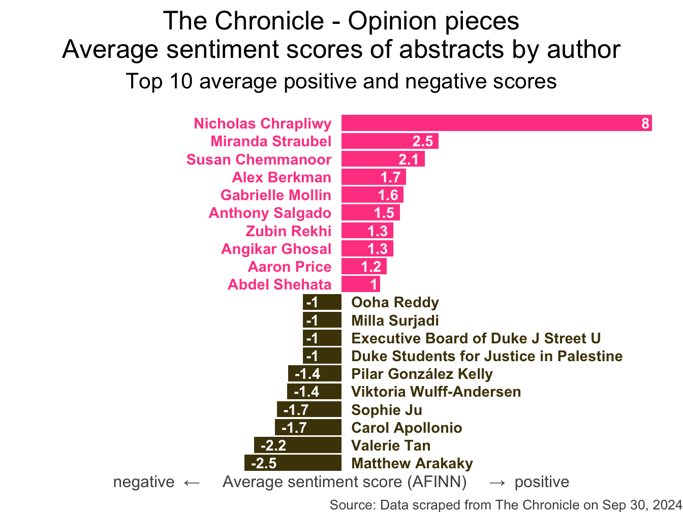
How do you think the sentiments in opinion pieces in The Chronicle compare across authors? Roughly the same? Wildly different? Somewhere in between?

Analyzing The Chronicle

All of this analysis is done in R!

(mostly) with tools you already know!

Common words in The Chronicle titles

Code for the earlier plot:

stop_words <- read_csv("data/stop-words.csv")
chronicle |>
  tidytext::unnest_tokens(word, title) |>
  mutate(word = str_replace_all(word, "’", "'")) |>
  anti_join(stop_words) |>
  count(word, sort = TRUE) |>
  filter(word != "duke's") |>
  slice_head(n = 20) |>
  mutate(word = fct_reorder(word, n)) |>
  ggplot(aes(y = word, x = n, fill = log(n))) +
  geom_col(show.legend = FALSE) +
  theme_minimal(base_size = 16) +
  labs(
    x = "Number of mentions",
    y = "Word",
    title = "The Chronicle - Opinion pieces",
    subtitle = "Common words in the 500 most recent opinion pieces",
    caption = "Source: Data scraped from The Chronicle on Sep 30, 2024"
  ) +
  theme(
    plot.title.position = "plot",
    plot.caption = element_text(color = "gray30")
  )

Avg sentiment scores of abstracts

Code for the earlier plot:

afinn_sentiments <- read_csv("data/afinn-sentiments.csv")
chronicle |>
  tidytext::unnest_tokens(word, abstract) |>
  mutate(word = str_replace_all(word, "’", "'")) |>
  anti_join(stop_words) |>
  left_join(afinn_sentiments) |> 
  group_by(author, title) |>
  summarize(total_sentiment = sum(value, na.rm = TRUE), .groups = "drop") |>
  group_by(author) |>
  summarize(
    n_articles = n(),
    avg_sentiment = mean(total_sentiment, na.rm = TRUE),
  ) |>
  filter(n_articles > 1 & !is.na(author)) |>
  arrange(desc(avg_sentiment)) |>
  slice(c(1:10, 40:49)) |>
  mutate(
    author = fct_reorder(author, avg_sentiment),
    neg_pos = if_else(avg_sentiment < 0, "neg", "pos"),
    label_position = if_else(neg_pos == "neg", 0.25, -0.25)
  ) |>
  ggplot(aes(y = author, x = avg_sentiment)) +
  geom_col(aes(fill = neg_pos), show.legend = FALSE) +
  geom_text(
    aes(x = label_position, label = author, color = neg_pos),
    hjust = c(rep(1,10), rep(0, 10)),
    show.legend = FALSE,
    fontface = "bold"
  ) +
  geom_text(
    aes(label = round(avg_sentiment, 1)),
    hjust = c(rep(1.25, 10), rep(-0.25, 10)),
    color = "white",
    fontface = "bold"
  ) +
  scale_fill_manual(values = c("neg" = "#4d4009", "pos" = "#FF4B91")) +
  scale_color_manual(values = c("neg" = "#4d4009", "pos" = "#FF4B91")) +
  coord_cartesian(xlim = c(-8, 8)) +
  labs(
    x = "negative  ←     Average sentiment score (AFINN)     →  positive",
    y = NULL,
    title = "The Chronicle - Opinion pieces\nAverage sentiment scores of abstracts by author",
    subtitle = "Top 10 average positive and negative scores",
    caption = "Source: Data scraped from The Chronicle on Sep 30, 2024"
  ) +
  theme_void(base_size = 16) +
  theme(
    plot.title = element_text(hjust = 0.5),
    plot.subtitle = element_text(hjust = 0.5, margin = unit(c(0.5, 0, 1, 0), "lines")),
    axis.title.x = element_text(color = "gray30", size = 12),
    plot.caption = element_text(color = "gray30", size = 10)
  )

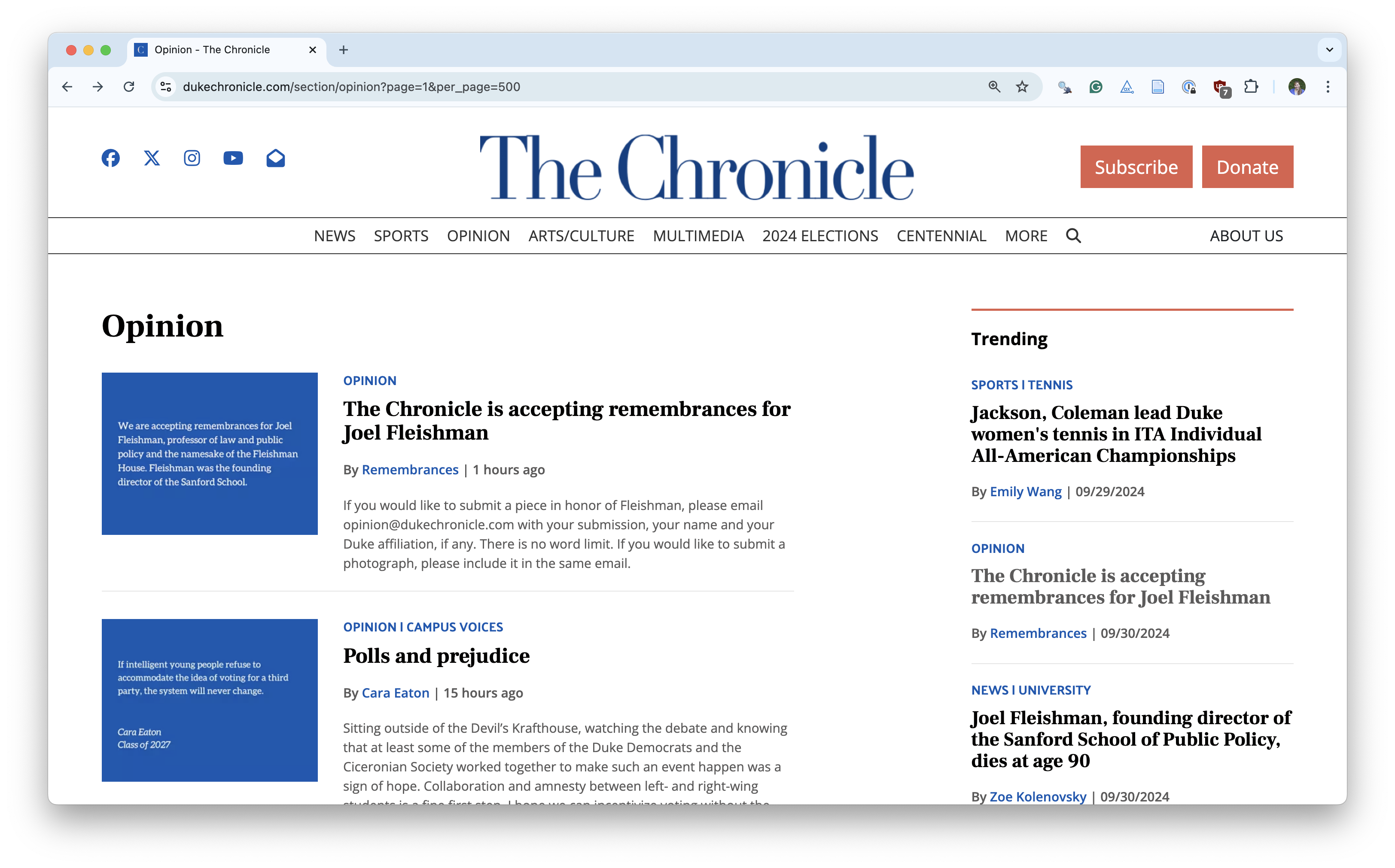
Where is the data coming from?

https://www.dukechronicle.com/section/opinion

Where is the data coming from?

chronicle

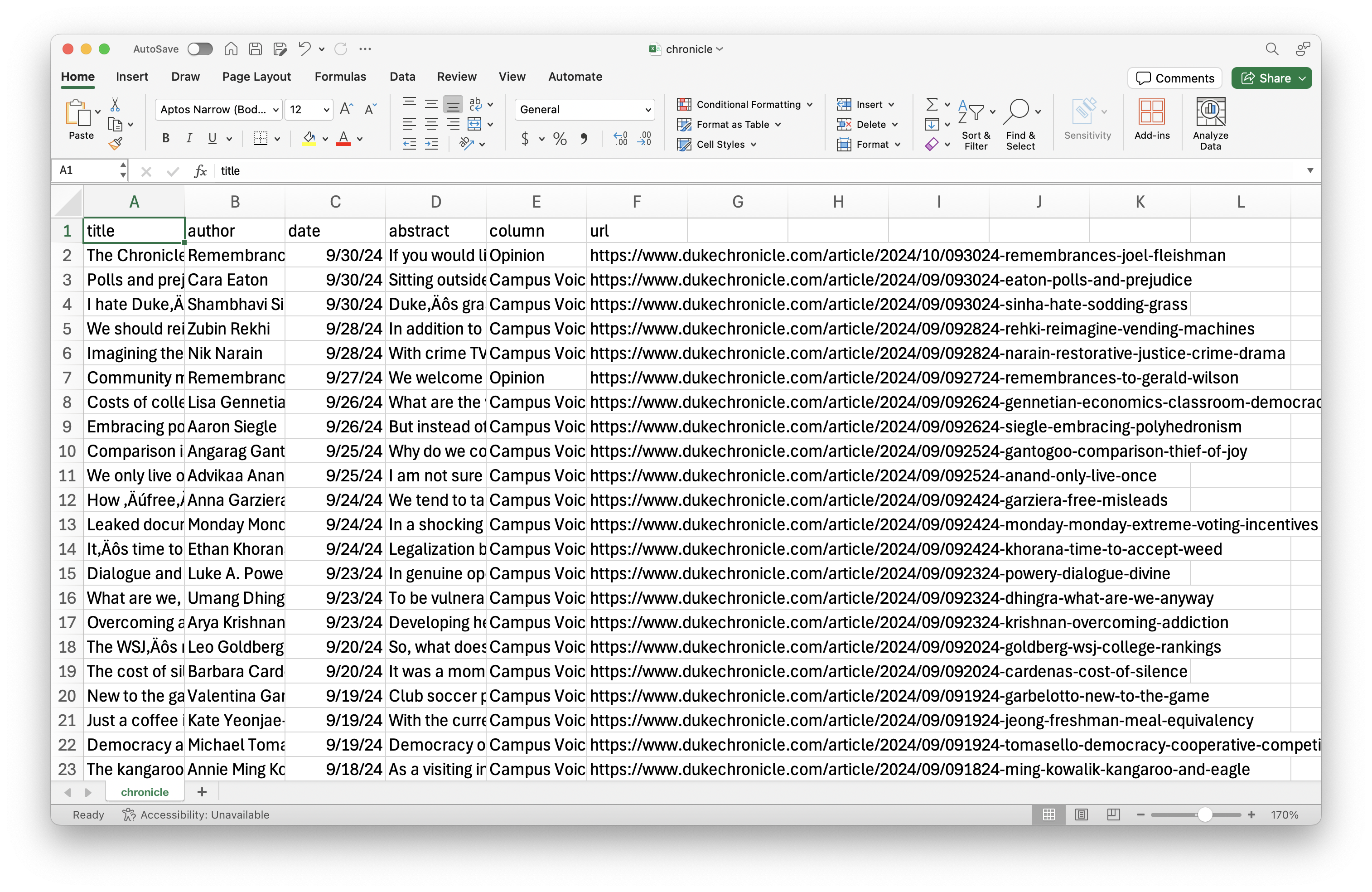
# A tibble: 500 × 6
   title                       author date       abstract column url  
   <chr>                       <chr>  <date>     <chr>    <chr>  <chr>
 1 The Chronicle is accepting… Remem… 2024-09-30 If you … Opini… http…
 2 Polls and prejudice         Cara … 2024-09-30 Sitting… Campu… http…
 3 I hate Duke’s sodding grass Shamb… 2024-09-30 Duke’s … Campu… http…
 4 We should reimagine our ve… Zubin… 2024-09-28 In addi… Campu… http…
 5 Imagining the restorative … Nik N… 2024-09-28 With cr… Campu… http…
 6 Community members share re… Remem… 2024-09-27 We welc… Opini… http…
 7 Costs of college campus ec… Lisa … 2024-09-26 What ar… Campu… http…
 8 Embracing polyhedronism     Aaron… 2024-09-26 But ins… Campu… http…
 9 Comparison is the thief of… Angar… 2024-09-25 Why do … Campu… http…
10 We only live once: Protect… Advik… 2024-09-25 I am no… Campu… http…
# ℹ 490 more rows

Web scraping

Scraping the web: what? why?

Increasing amount of data is available on the web
These data are provided in an unstructured format: you can always copy&paste, but it’s time-consuming and prone to errors
Web scraping is the process of extracting this information automatically and transform it into a structured dataset
Two different scenarios:
- Screen scraping: extract data from source code of website, with html parser (easy) or regular expression matching (less easy).
- Web APIs (application programming interface): website offers a set of structured http requests that return JSON or XML files.

Hypertext Markup Language

Most of the data on the web is still largely available as HTML - while it is structured (hierarchical) it often is not available in a form useful for analysis (flat / tidy).

<html>
  <head>
    <title>This is a title</title>
  </head>
  <body>
    <p align="center">Hello world!</p>
    <br/>
    <div class="name" id="first">John</div>
    <div class="name" id="last">Doe</div>
    <div class="contact">
      <div class="home">555-555-1234</div>
      <div class="home">555-555-2345</div>
      <div class="work">555-555-9999</div>
      <div class="fax">555-555-8888</div>
    </div>
  </body>
</html>

rvest

The rvest package makes basic processing and manipulation of HTML data straight forward
It’s designed to work with pipelines built with |>
rvest.tidyverse.org

library(rvest)

rvest

Core functions:

read_html() - read HTML data from a url or character string.
html_elements() - select specified elements from the HTML document using CSS selectors (or xpath).
html_element() - select a single element from the HTML document using CSS selectors (or xpath).
html_table() - parse an HTML table into a data frame.
html_text() / html_text2() - extract tag’s text content.
html_name - extract a tag/element’s name(s).
html_attrs - extract all attributes.
html_attr - extract attribute value(s) by name.

html, rvest, & xml2

html <- 
'<html>
  <head>
    <title>This is a title</title>
  </head>
  <body>
    <p align="center">Hello world!</p>
    <br/>
    <div class="name" id="first">John</div>
    <div class="name" id="last">Doe</div>
    <div class="contact">
      <div class="home">555-555-1234</div>
      <div class="home">555-555-2345</div>
      <div class="work">555-555-9999</div>
      <div class="fax">555-555-8888</div>
    </div>
  </body>
</html>'

read_html(html)

{html_document}
<html>
[1] <head>\n<meta http-equiv="Content-Type" content="text/html; cha ...
[2] <body>\n    <p align="center">Hello world!</p>\n    <br><div cl ...

Selecting elements

read_html(html) |> html_elements("p")

{xml_nodeset (1)}
[1] <p align="center">Hello world!</p>

read_html(html) |> html_elements("p") |> html_text()

[1] "Hello world!"

read_html(html) |> html_elements("p") |> html_name()

[1] "p"

read_html(html) |> html_elements("p") |> html_attrs()

[[1]]
   align 
"center"

read_html(html) |> html_elements("p") |> html_attr("align")

[1] "center"

More selecting tags

read_html(html) |> html_elements("div")

{xml_nodeset (7)}
[1] <div class="name" id="first">John</div>
[2] <div class="name" id="last">Doe</div>
[3] <div class="contact">\n      <div class="home">555-555-1234</di ...
[4] <div class="home">555-555-1234</div>
[5] <div class="home">555-555-2345</div>
[6] <div class="work">555-555-9999</div>
[7] <div class="fax">555-555-8888</div>

read_html(html) |> html_elements("div") |> html_text()

[1] "John"                                                                                  
[2] "Doe"                                                                                   
[3] "\n      555-555-1234\n      555-555-2345\n      555-555-9999\n      555-555-8888\n    "
[4] "555-555-1234"                                                                          
[5] "555-555-2345"                                                                          
[6] "555-555-9999"                                                                          
[7] "555-555-8888"

CSS selectors

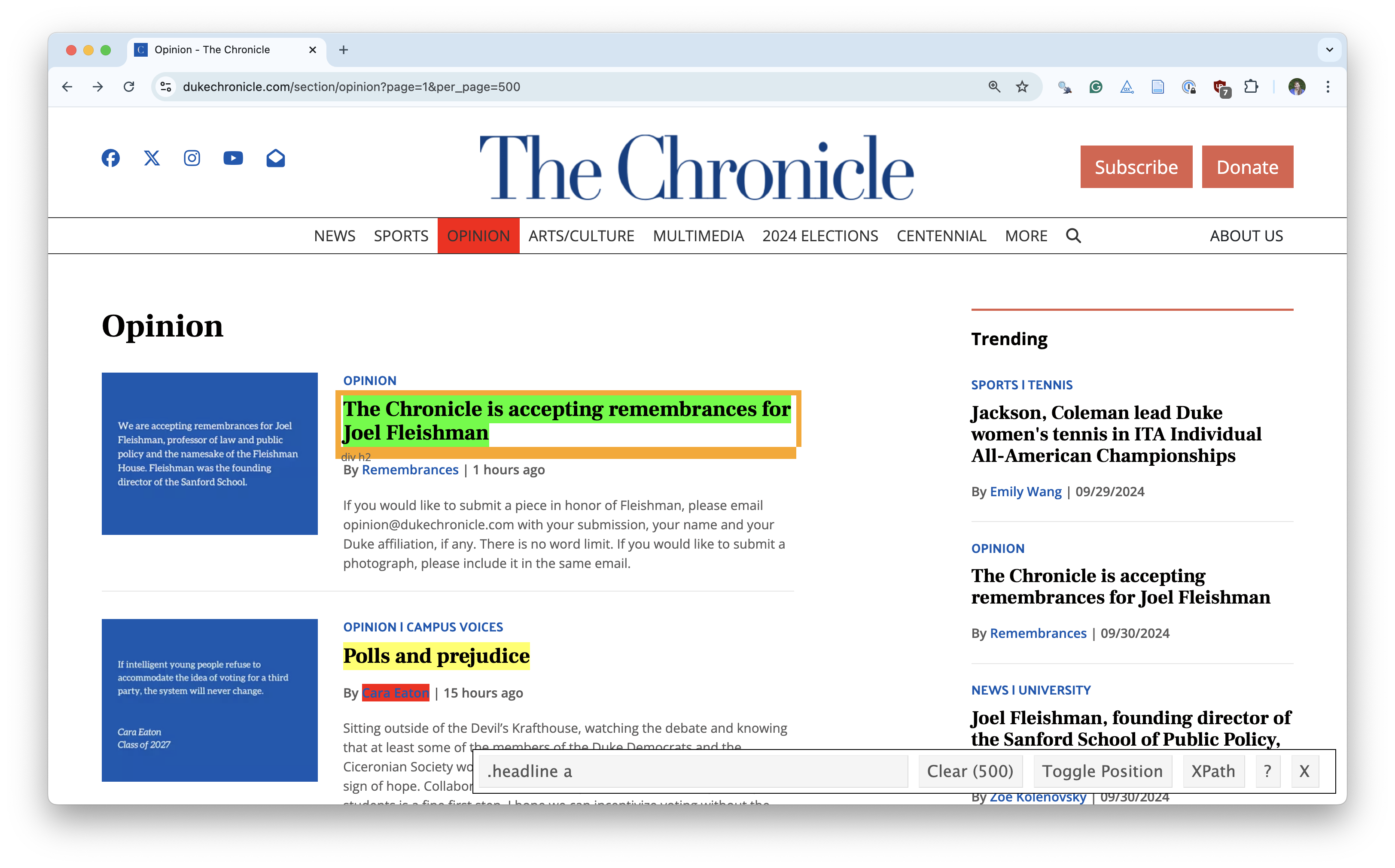
We will use a tool called SelectorGadget to help us identify the HTML elements of interest by constructing a CSS selector which can be used to subset the HTML document.

Some examples of basic selector syntax is below,

Selector	Example	Description
.class	`.title`	Select all elements with class=“title”
#id	`#name`	Select all elements with id=“name”
element	`p`	Select all <p> elements
element element	`div p`	Select all <p> elements inside a <div> element
element>element	`div > p`	Select all <p> elements with <div> as a parent
[attribute]	`[class]`	Select all elements with a class attribute
[attribute=value]	`[class=title]`	Select all elements with class=“title”

CSS classes and ids

read_html(html) |> html_elements(".name")

{xml_nodeset (2)}
[1] <div class="name" id="first">John</div>
[2] <div class="name" id="last">Doe</div>

read_html(html) |> html_elements("div.name")

{xml_nodeset (2)}
[1] <div class="name" id="first">John</div>
[2] <div class="name" id="last">Doe</div>

read_html(html) |> html_elements("#first")

{xml_nodeset (1)}
[1] <div class="name" id="first">John</div>

Text with `html_text()` vs. `html_text2()`

html = read_html(
  "<p>  
    This is the first sentence in the paragraph.
    This is the second sentence that should be on the same line as the first sentence.<br>This third sentence should start on a new line.
  </p>"
)

html |> html_text()

[1] "  \n    This is the first sentence in the paragraph.\n    This is the second sentence that should be on the same line as the first sentence.This third sentence should start on a new line.\n  "

html |> html_text2()

[1] "This is the first sentence in the paragraph. This is the second sentence that should be on the same line as the first sentence.\nThis third sentence should start on a new line."

HTML tables with `html_table()`

html_table = 
'<html>
  <head>
    <title>This is a title</title>
  </head>
  <body>
    <table>
      <tr> <th>a</th> <th>b</th> <th>c</th> </tr>
      <tr> <td>1</td> <td>2</td> <td>3</td> </tr>
      <tr> <td>2</td> <td>3</td> <td>4</td> </tr>
      <tr> <td>3</td> <td>4</td> <td>5</td> </tr>
    </table>
  </body>
</html>'

read_html(html_table) |>
  html_elements("table") |> 
  html_table()

[[1]]
# A tibble: 3 × 3
      a     b     c
  <int> <int> <int>
1     1     2     3
2     2     3     4
3     3     4     5

SelectorGadget

SelectorGadget (selectorgadget.com) is a javascript based tool that helps you interactively build an appropriate CSS selector for the content you are interested in.

Application exercise

Opinion articles in The Chronicle

Go to https://www.dukechronicle.com/section/opinion?page=1&per_page=500.

How many articles are on the page?

Goal

Scrape data and organize it in a tidy format in R
Perform light text parsing to clean data
Summarize and visualze the data

ae-10-chronicle-scrape

Go to your ae project in RStudio.
If you haven’t yet done so, make sure all of your changes up to this point are committed and pushed, i.e., there’s nothing left in your Git pane.
If you haven’t yet done so, click Pull to get today’s application exercise file: ae-10-chronicle-scrape.qmd and chronicle-scrape.R.

Recap

Use the SelectorGadget identify tags for elements you want to grab
Use rvest to first read the whole page (into R) and then parse the object you’ve read in to the elements you’re interested in
Put the components together in a data frame (a tibble) and analyze it like you analyze any other data

A new R workflow

When working in a Quarto document, your analysis is re-run each time you knit
If web scraping in a Quarto document, you’d be re-scraping the data each time you knit, which is undesirable (and not nice)!
An alternative workflow:
- Use an R script to save your code
- Saving interim data scraped using the code in the script as CSV or RDS files
- Use the saved data in your analysis in your Quarto document

Web scraping considerations

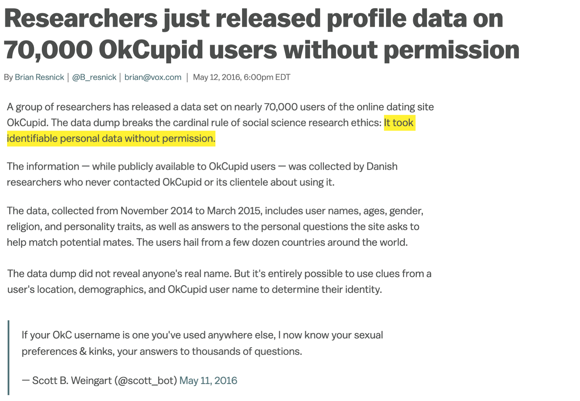
Ethics: “Can you?” vs “Should you?”

“Can you?” vs “Should you?”

Challenges: Unreliable formatting

Challenges: Data broken into many pages

Workflow: Screen scraping vs. APIs

Two different scenarios for web scraping:

Screen scraping: extract data from source code of website, with html parser (easy) or regular expression matching (less easy)
Web APIs (application programming interface): website offers a set of structured http requests that return JSON or XML files

Web scaping

Warm-up

While you wait…

Announcements

From last time

Age gaps

Age gaps

Age gaps

Age gaps

Data on the web

Reading The Chronicle

Reading The Chronicle

Analyzing The Chronicle

Reading The Chronicle

Analyzing The Chronicle

All of this analysis is done in R!

Common words in The Chronicle titles

Avg sentiment scores of abstracts

Where is the data coming from?

Where is the data coming from?

Web scraping

Scraping the web: what? why?

Hypertext Markup Language

rvest

rvest

html, rvest, & xml2

Selecting elements

More selecting tags

CSS selectors

CSS classes and ids

Text with html_text() vs. html_text2()

HTML tables with html_table()

SelectorGadget

Application exercise

Opinion articles in The Chronicle

Goal

ae-10-chronicle-scrape

Recap

A new R workflow

Web scraping considerations

Ethics: “Can you?” vs “Should you?”

“Can you?” vs “Should you?”

Challenges: Unreliable formatting

Challenges: Data broken into many pages

Workflow: Screen scraping vs. APIs

Text with `html_text()` vs. `html_text2()`

HTML tables with `html_table()`